
Satellite Image Analysis
25 Nov 2017
Find similar regions in satellite images by implementing singular value decomposition and locality sensitive hashing from scratch. Dataset
Table of contents
1. Goal
The Goal of this post is to analyse the Satellite Images GeoTIFF file of Long Island Area. The main objectives of this post is to implement Locality Sensitive Hashing and dimensionality reduction to get further experience with Spark and data preprocessing and explore a different modality of data: Satellite Images. I would be using numpy as much as possible because of its speed over default lists and tuple available in python. The speedup against python collections is immense here, where I was able to complete the entire task in 5 mins, where as the same using python collections took more than 1.5 hours in the same AWS environment.
To reduce the overhead of large images, we will split it into smaller images. Next part would be to flatten images to a 1d vector, preserving the spatial information of images. Having the image as a single large feature vector, we use LSH to group similar images. Finally we use dimensionality reduction using PCA and using these smaller feature vectors, find nearest images in each group found using LSH.
2. Dataset
The Data consists of high resolution orthorectified satellite images. Orthorectified images satellite pictures which have been corrected for abnormalities due to tilt in photography or geography. As mentioned here
High resolution orthorectified images combine the image characteristics of an aerial photograph with the geometric qualities of a map. An orthoimage is a uniform-scale image where corrections have been made for feature displacement such as building tilt and for scale variations caused by terrain relief, sensor geometry, and camera tilt. A mathematical equation based on ground control points, sensor calibration information, and a digital elevation model is applied to each pixel to rectify the image to obtain the geometric qualities of a map.

A digital orthoimage may be created from several photographs mosaicked to form the final image. The source imagery may be black-and-white, natural color, or color infrared with a pixel resolution of 1-meter or finer. With orthoimagery, the resolution refers to the distance on the ground represented by each pixel.

Georeferenced orthoimages support a variety of geographic information analysis and mapping applications, and provide the foundation for most public and private Geographic Information Systems.
We are using only the images of the Long Island area, and they consist of roughly around 50 Zipped TIFF Files. The images are of 2500x2500 or 5000x5000 resolution. Each pixel is 4-size array indicating 4 components [Red, Green, Blue, Infrared].
3. Reading Images
3.1. Convert Images to array
As our dataset consists of files as zip file, we would like to read the zip file, and return the tiff file enclosed within the zip as array.
We are using this method for doing the same. The code is pretty self explanatory. The returned array is of size (image-width, image-height, 4) where the 3rd dimension of the array specifies (R, G, B, Infrared) components.
def getOrthoTif(zfBytes):
    # given a zipfile as bytes (i.e. from reading from a binary file),
    # return a np array of rgbx values for each pixel
    bytesio = io.BytesIO(zfBytes)
    zfiles = zipfile.ZipFile(bytesio, "r")
    # find tif:
    for fn in zfiles.namelist():
        if fn[-4:] == '.tif':  # found it, turn into array:
            tif = TiffFile(io.BytesIO(zfiles.open(fn).read()))
            return tif.asarray()
I am reading the zip files from an HDFS using spark’s binaryfiles method and apply it to each zip file:
rdd_1a = sc.binaryFiles('./*.zip')
rdd_1b = rdd_1a.map(lambda x: (x[0], getOrthoTif(x[1])))s
The output would look like
‘/data/ortho/small_sample/3677453_2025190.zip’, [image as array]
3.2. Splitting Images
Since the images are around 25 mb each, they take time to load and are a bit heavy. Hence we split them into smaller sized images.
I divide the image into 25( from 2500x2500 images) or 100 (from 5000x5000 images) even sized images of resolution 500x500 using numpy.split. First I split the images horizontally using:
new_size = 500
factor = int(img.shape[0]/new_size)
y = np.array(np.split(img, factor, 1))
and then verically using:
y = np.array(np.split(y, factor, 1))
and then reshape the result of the previous split to get a flat array of 25 or 100 subimages using:
z = y.reshape([y.shape[0]*y.shape[1]]+list(y.shape[2:]))
Now z contains all the subimages. I change the filenames to contain both file name and the sub image part number. I convert all the images to pairs of (file-name-with-part-number, subimage). Combining all them into a method:
def split_images(name, img, new_size=500):
    factor = int(img.shape[0]/new_size)
    file_name = name.split('/')[-1]
#     print(factor)
#     x = rdd_tiff_array.take(1)[0][1]
    y = np.array(np.split(img, factor, 1))
    y = np.array(np.split(y, factor, 1))
    z = y.reshape([y.shape[0]*y.shape[1]]+list(y.shape[2:]))
    result = list()
    for i, arr in enumerate(z):
        result.append((file_name+'-'+str(i), arr))
    return result
I use this method to convert the filename, image to smaller images using spark:
rdd_1d = rdd_1b.flatMap(lambda x: split_images(x[0], x[1]))
Checking an intermediate result:
x = rdd_1d.filter(lambda x: '-0' in x[0]).first()
print("Filename:",x[0])
plt.imshow(x[1])
plt.show()
Output:
Filename: 3677454_2025195.zip-0
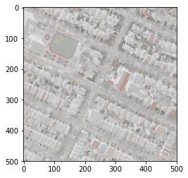
This output is the first subimage for the tiff file in 3677454_2025195.zip of size 500x500.
4. Feature Vector from Images
4.1. Reducing resolution of images
For similarity search we need to convert these images to represent them as a feature vector. Directly flattening the image into a single long vector is not a good idea as we will lose spatial information within images. Hence we need to perform some operations on the images to make it a single vector.
First step would be to converting the pixel array of RGBI values to just one value, i.e, intensity of each pixel. I used the following function:
intensity = int(rgb_mean * (infrared/100))
I take the mean of the first 3 components of the image’s along the 2nd axis(the 2nd axis contains the rgbi array), and then take out the intensity of each pixel.
def convert_to_one_channel(img):
    img = img.astype(np.float)
    x = np.mean(img[:, :, :3], axis=2)*img[:,:,3]/100
#     plt.imshow(x)
#     plt.show()
    return x
I use this method as an argument to map on all subimages.
rdd_2a = rdd_1d.map(lambda x: (x[0], convert_to_one_channel(x[1])))
The result:
plt.imshow(rdd_2a.first()[1])
plt.show()
Output:
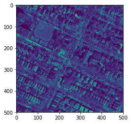
This image is a single channel with intensity value of each pixel. (The image is colored because I didn’t pass argument to plt.imshow() to make it grayscale).
We also reduce the resolution of the subimage to a size 50x50 by using an average operator. I split the image first vertically and then split the result of the previous split horizontally, getting a 50x50x10x10 array. Then, I take the average over these 10x10 cells to get the reduced resolution image.
def reduce_resolution(img, factor=10):
    section_size = img.shape[0]/factor
    y = np.array(np.split(img, section_size, 1))
    y = np.array(np.split(y, section_size, 1))
    z = np.mean(y, axis=(2,3))
    return z
I map this method to all 500x500 subimages.
rdd_2b = rdd_2a.map(lambda x: (x[0], reduce_resolution(x[1])))
Output:

4.2. Images as 1-d vector
The direct intensity value are not useful but rather how each pixel changes from one pixel to next. So we will be using row difference and column difference of the image as our new image. Also we clip these values to three values: -1,0,1 to represent the direction of change.
I used np.diff, np.where and np.clip to perform these changes.
- np.diff computes the difference along a specific axis
arr = np.diff(arr, axis=axis) - np.where to change all values between -1 to 1 as 0
arr = np.where(np.logical_or(arr<-1, arr>1), arr, 0) - and finally clip all values to -1 and 1, hence changing the matrix into only values with -1,0 and 1.
arr = np.clip(arr, -1, 1)
I reshape the image to two 49x50 array to represent row_diff and col_diff and horizontally stack them into a single 4900 size feature vector.
def convert_values(arr, axis):
    arr = np.diff(arr, axis=axis)
    arr = np.where(np.logical_or(arr<-1, arr>1), arr, 0)
    arr = np.clip(arr, -1, 1)
    arr = arr.reshape(arr.shape[0]*arr.shape[1])
    return arr

rdd_2e = rdd_2b.map(lambda x: (x[0], np.hstack((convert_values(x[1], 1), (convert_values(x[1], 0))))))
This results in subimages being flattened into 4900 dimensions 1d vector. Now we can proceed to similarity search.
5. Finding Similar images from PCA, LSH
5.1. Locality Sensitive Hashing
Locality sensitive hashing(LSH) is a really helpful concept when looking for similar objects. Without LSH we have to check the similarity with all possible object for a given queried object. But many of the objects can be rejected by clustering objects into similar group. These groups can have false positives but the probability is pretty low.
Seeing how LSH works might help in visualising it more. In LSH, we first split objects into smaller bands and we group any object that are exactly similar in any of the band. This results in groups that were similar to any object in atleast one of the band. This reduces the search space by a lot. And in this reduced search space, we can use any distance measure to get the most similar objects to a given query object by sorting them according to their distance.
We can also control the false positives by decreasing the number of splits, due to which only those elements will go to a group which are identical even in these large band.
Also to look for identical parts, we use hash functions. We hash bands into buckets, and if the hash values of same bands of different images are same, we place them in the same group. The more the number of the buckets or hash values are there, there is smaller probability of hash collision, and hence lesser is the false positive rate.
Though there are libraries to do this in spark, here we do it without any library to learn how it works.
We first change the feature vector into a 128 byte signature vector from the 4900 size feature vector:
def create_signature(vec):
    vec_arr = np.array_split(vec, 128)
    result = list()
    for item in vec_arr:
        a = hashlib.md5(item)
        b = a.hexdigest()
        as_int = int(b, 16)
        result.append(as_int%2)
    return 1*np.array(result, dtype=np.bool)

rdd_3a = rdd_2e.map(lambda x: (x[0], create_signature(x[1])))
Each image now is represented into a 128 byte vector. I am using np.array_split which splits arrays into similar sized splits of 38/39 features.
We then split the 128 byte signature vector into 16 bands. For each band, we calculate the bucket number using a hash function and make a tuple for each subimage:
((band-number, bucket-number), image-name)
The key being (band-number, bucket-number).
If we group by using this key, we would get all images that have the same bucket number for the same band-number.
def LSH(vec, bands=16, buckets=671):
    band_split = np.split(vec, bands)
    result = []

    for i,bi in enumerate(band_split):
        a = hashlib.md5(band_split[0])
        b = a.hexdigest()
        result.append((i, hash(np.array_str(bi))% buckets))
    return result
We use this method and apply to:
rdd_3b_1 = rdd_3a.flatMap(lambda x: [(item, x[0]) for item in LSH(x[1])]).groupByKey().mapValues(list)
This RDD now contains all images that go into the same bucket for the same band.
Now for each image, we make groups of images that are similar to that image.
rdd_3b = rdd_3b_1.flatMap(lambda x: [(item, x[1]) for item in x[1]]).reduceByKey(lambda a,b: list(set(a+b)))
The resultant tuple would be
(image, set-of-images-similar-to-this-image)
5.2. Dimensionality Reduction using PCA(SVD)
Now that we have got flattened images, and group of images that are similar to it, we can use it to search for similar images within the group. But the problem lies in such large feature size images of 4900 dimensions. Not all the features are important and some of them can be ignored while computing for closeness between two images.
So we use a very common dimensionality reduction technique, called principal component analysis. In principal component analysis, we chose only the most varying features and give lower importance that show less variability over the entire sample space.
Using the most significant principal component reduces the dimensionality of a feature vector, yet preserving a lot of the variation in the dataset. The more number of principal components leads to a better representation of the original dataset. To read more about this, please go to this link.
Singular Value Decomposition is one way to perform PCA on the images and we are going to use the same here. We are going to use the linalg SVD method of numpy library. This method gives us the three matrix required to compute SVD of any vector of the dataset.
Now the main challenge is applying SVD over a distributed network. We can apply the SVD method over the entire data. But that would be both unnecessary and defeats the purpose, because collecting over such a large dataset and applying SVD is really expensive.
We hence go with an approximation approach where we randomly sample from the subimages feature vector, compute the SVD matrix and then broadcast it to apply it over all the images. This Incremental method was proposed in:
Sarwar, Badrul, et al. “Incremental singular value decomposition algorithms for highly scalable recommender systems.” Fifth International Conference on Computer and Information Science. Citeseer, 2002.
First step would be to take a sample of 500 items and compute SVD based on these 500 items. I broadcasted the U, s and Vh obtained from the linalg.SVD method to use it to transform all feature vector to reduced size using only the first 10 principal components.
def getSVD(arr, dimens=10):
    global broadcast_mu, broadcast_std, broadcast_Vh
    mat = np.zeros((len(arr), arr[0][1].shape[0]), dtype=np.float)
    for i,l in enumerate(arr):
        mat[i] = np.array(l[1])
    mu, std = np.mean(mat, axis=0), np.std(mat, axis=0)
    mat_zs = (mat - mu) / std
    U, s, Vh = np.linalg.svd(mat_zs, full_matrices=0)
    broadcast_mu = sc.broadcast(mu)
    broadcast_std = sc.broadcast(std)
    broadcast_Vh = sc.broadcast(Vh[:dimens].T)
    return

batch = rdd_2e.takeSample(500, false)
getSVD(batch)
Once computed and broadcasted, I use the following method to transform the image’s feature vector:
def transform(feature):
    feature_zs = (feature-broadcast_mu.value) / broadcast_std.value
    t1 = np.dot(feature_zs, broadcast_Vh.value)
    t2 = np.matmul(feature_zs, broadcast_Vh.value)
    return np.dot(feature_zs, broadcast_Vh.value)

rdd_3c_0 = rdd_2e.map(lambda x: (x[0], transform(x[1])))
I also join the reduced feature vector of size 10 with the group of similar for an image
rdd_3c_1 = rdd_3b.join(rdd_3c_0).flatMap(lambda x: [(item, (x[0],x[1][1])) for item in x[1][0] if item!=x[0]])
Now the output should look like this:
(file-name, (image-feature-vector, set-of-images-to-this-image))
Then I calculate the distance between each image and sort to get a RDD of top close images for each image.
def distance(d1, d2):
    return np.linalg.norm(d1-d2)

rdd_3c_2 = rdd_3c_1.join(rdd_3c_0).map(lambda x: (x[1][0][0], (x[0], distance(x[1][0][1],x[1][1]))))

rdd_3c_3 = rdd_3c_2.groupByKey().mapValues(list)

def sort_by_dist(pair):
    key, value = pair
    value.sort(key=lambda t: t[1])
    return key, value
rdd_3c = rdd_3c_3.map(sort_by_dist)
6. Results
To get the top 10 images close to any queried image we can use the following code:
rdd_3c_1 = rdd_3c.filter(lambda x: '3677454_2025195.zip-1'==x[0])
pprint.pprint(rdd_3c_1.first()[1])
Output:
[(‘3677500_2035190.zip-17’, 50.601650444294656), (‘3677502_2035200.zip-6’, 51.6015513800319), (‘3677453_2025190.zip-0’, 52.286280183298871), (‘3677502_2035200.zip-13’, 52.919475348704736), (‘3677501_2035195.zip-7’, 53.161931352632621), (‘3677453_2025190.zip-20’, 53.217692458807115), (‘3677453_2025190.zip-9’, 53.41184799850511), (‘3677502_2035200.zip-22’, 53.557952615702291), (‘3677453_2025190.zip-12’, 53.596719688352465), (‘3677500_2035190.zip-6’, 55.151102107788134), (‘3677454_2025195.zip-17’, 57.096403314719502), (‘3677454_2025195.zip-20’, 66.134879053561022), (‘3677454_2025195.zip-3’, 83.487893878865549)]
These are the top 10 images closest to 3677454_2025195.zip-1 along with their distance from the queried image.
Visual output:
2 images closest to 3677454_2025195.zip-8 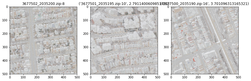
Thats It! Thanks for reading this post and feel free to look into the entire code in my github repo: Satellite Image Analysis to find similar regions using Spark