Table of contents

1. Goal
2. Dataset
3. Analysing and processing images
   1. Split Images to subimages
   2. Calculating feature vector
4. Clustering
   1. Elbow method
   2. Applying clusters in RDD
5. Similarity search
6. Results

1. Goal

This blog post is a part of our final project that was part of the coursework in CSE545. The project was based on United Nations sustainable development goals to ensure sustainable consumption and production patterns of natural resources using big data. Our project proposed of a method to tie in high quality data available in developed countries, such as the United States, to predict water consumption in other countries based on similarity with consumption pattern of states of the USA. We used two datasets Global Satellite Images for surface water analysis and USGS water dataset. We first predicted trends in the United States water consumption and also made a tool for given any coordinates anywhere in the world, it could locate which areas of the United States have similar surface water patterns.

This blog is focused on only on the part of similarity search of satellite images. There are mainly three parts of the task, first, the dataset analysis; secondly, cleaning of dataset to represent each coordinates using a small feature vector; and lastly, clustering images to find similar regions for any given coordinates.

2. Dataset

The Global Surface Water dataset shows different facets of the spatial and temporal distribution of surface water over the last 32 years. Some of these datasets are intended to be mapped (e.g. the seasonality layer) and some are intended to show the temporal change at specific locations (i.e. the water history). In addition, there are datasets that provide metadata on the number of observations and valid observations that were used and these can be used to estimate the confidence levels in the data.

We will be only using the dataset related to “Occurrence Change Intensity”. This dataset consists of global satellite images to represent the change in water occurrence intensity in two epochs: (16 March 1984 to 31 December 1999, and 1 January 2000 to 10 October 2015). As per the dataset description:

An example of the Occurrence Change Intensity dataset is shown below for the Brahmaputra River. Increases in water occurrence are shown in green and decreases are shown in red. Black areas are those areas where there is no significant change in the water occurrence during the 1984 -2015 period. The intensity of the color represents the degree of change (as a percentage). For example, bright red areas show greater loss of water than light red areas. Some areas appear grey in the maps, these are locationswhere there is insufficient data to compute meaningful change statistics

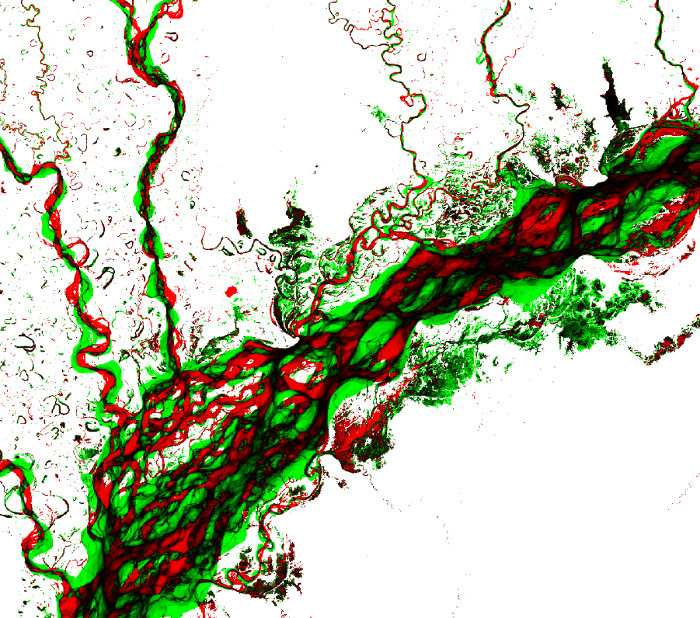
Intuitively, if we compute the area of image in black, red or green pixel, we get the amount of surface water area where there has been no change, lost water surface, and new water surfaces respectively, for each tile of land area. If we use these as features, we can use it for similarity search of regions with similar surface water trends.

So we divide the entire global image dataset into small tiles of regions, roughly each region having a span of 100 sq. km., compute the feature vector for each region, and use it for clustering of regions and similarity search.

3. Analysing and processing images

Too start with the task, we download the dataset from a script that is given here. All the images related to Occurrence Change Intensity are in the dataset labeled as change. After downloading it, the files are in the form of TIFF File with a size of around 42Mb each. Processing such a large file is both memory and performance intensive. So we first divide it into smaller parts and then compute the feature vector for each smaller sub images.

3.1 Split images to subimages

Since the dataset is quite large(~ 8gb of Tiff files), we used spark for a distributed way to solve the problem. Each tile was spanned a region of 10˚ in latitude and 10˚ in longitude (40,000x40,000 pixels). So we used PIL library and spark in python to divide the large tiff files into smaller tiles of 2000x2000 pixels size (spanning across 0.5˚ latitude and 0.5˚ longitude), encompassing approx. area of 100 sq. km.

To divide each image, we load each file using SparkContext.binaryFiles which reads each file as a binary file and returns an RDD with (file-name, file-as-binary-file) tuple. I am just using the file name here and using cv2.imread on the file-name to get the image.

Then having the image as a numpy array using cv2 imread, I split it into horizontally and vertically into 20x20 2000x2000 images.

factor = int(img.shape[0]/new_size)

w = np.split(img, factor, 1)
y1 = np.array(w)
w1 = np.split(y1, factor, 1)
y = np.array(w1)
z = y.reshape([y.shape[0]*y.shape[1] + list(y.shape[2:]))

The tricky part here is to compute the coordinates of the left corner of these small sub images. I split the file name: ex 110W_40N.tiff and extract coordinates of the 40000x40000 image, and assign a new coordinate to each new sub image. In case of W and N based coordinates, we need to subtract latitude/longitude as we go left-to-right/up-to-down in the image because we are approaching the 0, 0 coordinate. Similarly, we should add, when we have an E or S coordinate.

file_name = name.split('/')[-1]
diff = 10 / factor
result = list()
file_name = file_name[:-4]
lat = float(file_name.split('_')[1][:-1])
e_w = 1 if file_name.split('_')[1][-1]=='E' else -1
lng = float(file_name.split('_')[2][:-1])
n_s = 1 if file_name.split('_')[2][-1]=='S' else -1
    
complement_dirn = { 'S': 'N', 'N': 'S', 'E': 'W', 'W': 'E'}
for i, arr in enumerate(z):
    latitude = (lat+n_s*(i%y.shape[0]) * diff)
    longitude = (lng+e_w*(i//y.shape[0]) * diff)
    dirn_lat = file_name.split('_')[1][-1]
    dirn_lng = file_name.split('_')[2][-1]
    if latitude<0:
        latitude = -1*latitude
        dirn_lat = complement_dirn[dirn_lat]
    if longitude<0:
        longitude = -1*longitude
        dirn_lng = complement_dirn[dirn_lng]
    result.append((str(latitude)+dirn_lat+'-'+str(longitude)+dirn_lng, arr))

Note: As in this project I had only used images from 180W, 180N to 0,0, I did not handle the case of E or S coordinates.

Now my RDD looks has the following tuples:

(Coordinates of top left corner, Images spanning 0.5˚ latitude/longitude)

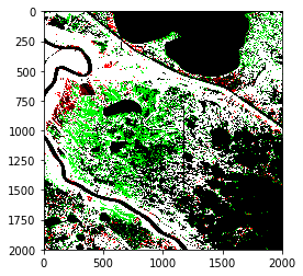
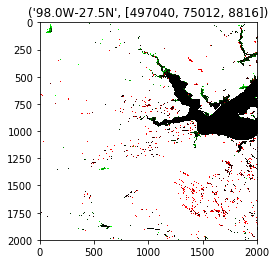
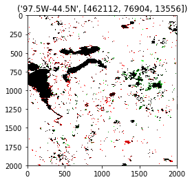
Some sample outputs:

Coordinates: ‘90.0W-30.0N’

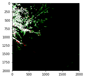
Coordinates: ‘89.5W-30.0N’

3.2 Calculating feature vectors

Within each tile, we counted the area of surface water lost permanently within each tile, surface water new found and area of water that remained unchanged. We used this data to create for each tile, a feature = (unchanged water area, lost water bodies, new found water bodies). We saved these into disks as text files for a reduced dataset to work on.

To calculate the feature vector, I counted the number of black pixel, red pixels and green pixels in each image. The number of pixel is directly proportional to the area of surface water unchanged, lost or new found in the duration of 1986-2016.

To calculate the area of each image, I used a pixel count method.

def pixel_count(x):
    name, img = x[0], x[1]
    black_px_count = np.argwhere(np.all(img==[0,0,0], axis = 2)).size
    red_px_count = np.argwhere(np.logical_and(img[:, :, 2]>50, img[:, :, 1]==0)).size
    green_px_count = np.argwhere(np.logical_and(img[:, :, 1]>50, img[:, :, 2]==0)).size
    return name, (black_px_count, red_px_count, green_px_count)

I then filtered the images which have neither any red nor green pixel.

rdd_filtered_images = rdd_1b.map(pixel_count).filter(lambda x: x[1][1]>0 or x[1][2]>0)

Now for each tile of 0.5˚ latitude-longitude, there is a feature vector with the relative area of unchanged, lost or new found surface water source visible in satellite images.

I save this computed feature vector as a new dataset using SparkContext.saveAsTextFile().

Sample output:

(‘90.0W-30.0N’, (3283034, 251530, 1107984))

(‘89.5W-30.0N’, (7214822, 28970, 232068))

4. Clustering

The feature vector here represents for each span of 0.5˚ in latitude and longitude, amount of change in surface water in this region. A region with lots of green pixel coverage has seen new sources of water, whereas region with red pixels have seen significant loss in water sources. Analysing these feature vectors represent different kinds of pattern in water trends. For ex. a region having a huge span of black area means regions with huge water sources, and regions that have higher ratio of red to green+red areas, means huge water sources have vanished over time. Similarly a larger ratio of green to red+green means that those regions have new found water sources. A 1:1 ratio of red to green areas represent change in location of water source and doesnt necessarily mean water scarcity or inundation.

Visualizing these feature vector in a 3d space shows points that show similar trends clustered together. Using K-means clustering, similar regions can be grouped based on the above analysis. We are using Spark’s mllib for the same.

4.1 Elbow method

In K-means clustering, all points are grouped around k points, each point being a mean of all the points in the cluster. As per pyspark mllib docs:

K-means is one of the most commonly used clustering algorithms that clusters the data points into a predefined number of clusters. The spark.mllib implementation includes a parallelized variant of the k-means++ method called kmeans||. The implementation in spark.mllib has the following parameters:

k is the number of desired clusters. Note that it is possible for fewer than k clusters to be returned, for example, if there are fewer than k distinct points to cluster.

maxIterations is the maximum number of iterations to run.
initializationMode specifies either random initialization or initialization via k-means||.

Deciding the number of clusters in k-means clustering is done using elbow method. In elbow method, the number of desired clusters is passed to the algorithm. We then compute Within Set Sum of Squared Error (WSSSE). We can reduce this error measure by increasing k. The optimal k is usually one where there is an elbow in the WSSSE vs k graph.

 def error(point):
        x = point[0]/(point[0]+point[1])
        y = point[1]/(point[0]+point[1])                    
        center = clusters.centers[clusters.predict((x, y))]
        return sqrt(sum([x**2 for x in (point - center)]))

for k in range(1, 20):
    clusters = KMeans.train(rdd_records.map(lambda x: (x[1][1]/(x[1][1]+x[1][2]), x[1][2]/(x[1][1]+x[1][2]))), k, maxIterations=12, initializationMode="random")  
    WSSSE = rdd_records.map(lambda x: error(x[1][1:])).reduce(lambda x, y: x + y)
    result.append(WSSSE)

plt.plot(result)
plt.show()

Output:

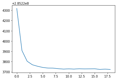
As per the elbow method analysis, k=10 is the optimal cluster in this case.

4.2 Applying clusters in RDD

Taking k=10, the entire dataset is clustered into 10 clusters. Firstly, we have to train a k-means model and then predict cluster for each feature tuple. Using the cluster number as key, we can group all images into a single RDD, and then perform similarity search within each cluster.

To train the model we use here from the Kmeans.train from mllib library, in which we pass rdd of all records with 2 features: ratio of red over red and green areas, and the second as green over red and green areas.

New feature vector: (coordinates, ( #-of-red-pixels / (#-of-green-pixels+#-red-pixels) , #-of-green-pixels / (#-of-green-pixels + #-of-red-pixels))

These ratios represent the amount of change in surface water bodies that were visible in the satellite images. This would allow us to group regions based on their relative amount of changes in the water bodies.

So we first map a transformation over each of the record to change the feature vector containing ratio of these red over red and green and green over red and green pixels. Then we train our k-means clustering model, using k=10 and 12 max iterations. We have also initialised the k-means cluster center as random points.

clusters = KMeans.train(rdd_records.map(lambda x: (x[1][1]/(x[1][1]+x[1][2]), x[1][2]/(x[1][1]+x[1][2]))), 10, maxIterations=12, initializationMode="random")

def cluster(point):
    u = point[1]/(point[1]+point[2])
    v = point[2]/(point[1]+point[2])
    return clusters.predict((u, v))

rdd_clusters = rdd_records.map(lambda x: (cluster(x[1]), x)).groupByKey().mapValues(list)

rdd_clusters holds all 10 clusters with coordinates grouped based on their similarities in red over red and green regions; and green over green and red regions.

5. Similarity search

For similarity search, we will use rdd_clusters. For any given coordinate, we round it to its nearest 0.5˚ latitude and longitude. Then we get its cluster index using the Kmeans.predict method. With the given cluster index, nearest neighbors are calculated according to our distance metric with relative ratios in red and green pixel as features.

We are using another library here, NearestNeighbors from spark mllib which returns the n nearest neighbors given all points in a cluster.

_, point = rdd_records.filter(lambda x: x[0]==query).first()
u = point[1]/(point[1]+point[2])
v = point[2]/(point[1]+point[2])
print(u,v, point)
cluster_num = clusters.predict((u, v))

cluster_points = rdd_clusters.filter(lambda x: x[0]==cluster_num).first()[1][1:]
knn = NearestNeighbors(n_neighbors=k)
points = [x[1][1:] for x in cluster_points]
knn.fit(points)
result = [cluster_points[idx] for idx in knn.kneighbors([point[1:]], return_distance=False)[0]]

6. Results

The final results:

Queried coordinates:

112.5W-41.0N [2579410, 1353330, 33720]

Output:

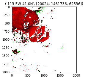
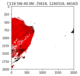
[(‘113.5W-41.0N’, [20024, 1461736, 62536]), (‘118.5W-40.0N’, [5618, 1240316, 4616]), (‘119.0W-43.5N’, [146486, 1482164, 6558]), (‘114.0W-41.5N’, [14440, 1147394, 10712]), (‘113.0W-41.5N’, [5097042, 1139238, 1026]), (‘113.5W-39.0N’, [260, 1019590, 860]), (‘119.0W-40.0N’, [13618, 1771930, 26888]), (‘120.0W-36.5N’, [11212, 852236, 37944])]

Visually the top 2 results for 2 different queries:

Query: 112.5W-41.0N

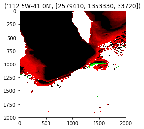
Top 2 outputs:

Query: 112.5W-41.0N

Top 2 outputs:

The results show similarity in the amount of surface area of water bodies changed in the past 30 years. Satellite images being available on a worldwide level could be then extended to tie the data from detailed dataset of USGS for US states to predict parameters like water quality and water depletion prediction for countries that dont have such infrastructure to directly infer these parameters.

Thanks for reading this post! You could check the github code in my repository: github-code